 Output Programming : Tables used to program the controller's outputs are set up here.
Voltages generated by output pins can also now be tested independently of external sensors.
Output Programming : Tables used to program the controller's outputs are set up here.
Voltages generated by output pins can also now be tested independently of external sensors.
Most controllers have three independently programmable hardware outputs of varying quality and maximum voltage.
Internal software tables program each output.
These tables are set up by this utility either as a simple linear relationship between Lambda/AFR and output voltage,
or a more complex relationship (up to 65 programmable points).
Note: The WBlin differential output is affected by the WBlin-GND
jumper/shunt hardware setting described here.
Note: Tech Edge displays do NOT use a voltage to display AFR/Lambda.
They use a digital value (Lambda16 or Ipx) from the controller.
Tables and Output PinsRefer to your controller documentation for each output pin's exact specifications. Not all outputs are at the same accuracy (WBlin is 12 bits on professional models, but only 9.5 bits on economy models), and not all outputs are available on all controllers. However, all outputs can be reprogrammed using WButil, and the output curve can be manually checked if you have a voltmeter (or use the target device connected to the voltage output). Basics : To re-program an output, first make sure the correct controller and sensor type is selected on the Controller Tab of the General page as this will change the selections available on the page shown at left as well as some of the raw programming parameters used. 
Now select the Output Pin to re-program - the example shows the WBlin output has been selected, and that WBlin uses a 12 bit (4095 individual steps over the voltage range) hardware DAC (Digital to Analogue Converter) - other outputs may use a lower quality PWM (Pulse Width Modulator) converter. The graph scale's Y axis (VOLTAGE) also changes with the maximum voltage available on the output pin.
Source and Axis SelectionThe Source Is selection determines the source of data to re-program the table. The example shows Linear Data Points have been selected - this allows simple straight line graphs to be easily created. Other options are Data From File and Predefined Table. These and more fully described below. 
The wideband controller is really a Lambda controller. Lambda can be directly converted to either AFR (Air-Fuel-Ratio), or % Oxygen (percent O2). The X Axis is menu selects this value to use, and attempts to convert the displayed data points from the currently selected value to the new value. This sometimes means a 1.0 will be converted to 0.9999 if repeated conversions are made. Also, a rich λ/AFR will be converted to a negative oxygen percentage and this will sometimes result in strange looking curves - we didn't try and fix these strange displays because it alerts you to the possibly "strange" data points present. 
The Stoich AFR value can only be set if AFR has been selected for the X-Axis. The relationship between Lambda and AFR depends on the Stoich AFR as shown in the box at left The correct Stoich AFR should be selected for your fuel if you want to re-program the outputs in native AFR units for your fuel. Source is : Linear Data Points
The image at right is for the Source Is Linear Data Points selection (and with X Axis AFR selected). It has four text boxes near the centre - they are organised vertically as (value, voltage) pairs. In this example value is AFR because the X-Axis has been selected as AFR. The lower text boxes are for entering the voltage on the output pin at each AFR point.
The second data point graph (above, main image) shows how 
Mid Points Used? : Apart from the two end points, one or two mid-points may be added to the graph using the Linear Data Points interface (there may be an n-point option in the future). The graph at left shows the 4 point option. The red line annotation matches the second data pair of data points (AFR=13.0 at V=1.8V) with the matching point on the graph.
Over/Under Volts? :
Graph Options
The graph can be resized by grabbing the lower right corner of the application, and dragging. The graph shows the most commonly re-programmed area of the controllers output - it does NOT show the range all the way to free-air on the λ & AFR selection, but does when Percent oxygen is selected. A Left mouse click on the graph will select the closest (nearest Ipx value) table cell, will highlight that Ipx value, and leave an indication of the point on the graph. A Right mouse click on the graph brings up the menu shown at right. The format and colour of many of the graph's elements can be customised as follows: Ipx Lines : are the vertical yellow bars on the graph. Each line represents a single table cell, with the value of the cell setting the output voltage point on each Ipx line. The curve's colour is set by the Ipx Line selection in the SET COLOURS section of the graph options. Ideal Curve : is the graph line that fits the requested data points exactly and is the dark blue line seen on some graphs. Because the data points are constrained to be on Ipx lines, the actual output voltage sometimes is not precisely what is desired. The line's colour is set by the Ideal Curve selection. Stoich Line : is the green line representing λ = 1.0 exactly. Note that it is between two Ipx lines and, for X Axis is AFR graphs, is at the point set in the Stoich AFR text box to the right of the X Axis is menu. The colour is set by the Stoich Reference selection. Show Controller Data : is displayed by the orange graph line when the table data from the controller has been read back using the [Read] button. The curve's colour is set by the Data from Unit selection. Source is : Data From FileA special file (.ipx format) may be used to re-program any of the outputs. We have not publicly document the format of this file yet. Source is : Predefined TablesSeveral predefined tables, set up in the .ini files supplied with WButil, can be selected and programmed into the controller. |
Writing/Saving Tables to the Controller
Of course, it's possible to set up a table without having the controller present, in which case you'll likely get an error message as shown here also - note the TIMEOUT message at the bottom left and the Write EE memory Error (truncated) message when trying to write the WBlin table. This was caused by selecting the wrong COM port (refer to the General Tab). In this case simply press the [Abort] button, and solve the communication problem.
|
Reading Controller TablesThe [Read] button can be used to either read the existing controller tables, or check that table data just written got there successfully. The Output Pin selection, as you would expect, determines the controller table that is read. The graph is updated to show both the read data and the data previously set automatically or by pressing the [Generate Table] button.It's important to note that WButil uses just one read/write buffer, so if you read data from a controller table then this overwrites whatever was in the buffer. This lets you fairly easily copy data from one controller to another by simply reading the data and writing it out again. Of course, if you change anything that causes the table to be rebuilt (such as altering one of the Linear Data Points or by pressing the [Generate Table] button, then the old data in the table will be lost. See below for a way to save data from a controller. 
Testing Output Table Voltages
This button is located to the right of the table display. Pressing it brings up the dialogue box shown at right. A short delay is required to set up the controller both entering and exiting this mode. note: first make sure the Over/Under Volts checkbox is not selected during this test. The controller should be in a test mode that produces a rapid three-flash status LED sequence to indicates the controller is ignoring sensor information. We can now independently set the DAC hardware's output voltage. The central slider adjusts the decimal DAC count between 0 and 4095. This count is shown in the text box under the slider, and a value may be entered directly into that text box. The arrow buttons change the count up, or down, by one. The DAC count is also shown in Hex (0x format) and the Data actually sent to the DAC is shown in Hex format too (note: 1472 decimal = 0x5C0). 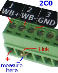
Along the top are a number of read-only text boxes displaying the count converted into other values. The top most values relate to Lambda which is calculated using a reverse table search (normally the tables convert Ipx or λ-16 to a DAC count) :
Just above the slider is the calculated Volts that can be measured between the external WBlin+ and WBlin- pins (see image at left). Remember, if you are using a voltmeter to measure this voltage, that a link MUST be used between the actual WBlin- and GND if the WBlin-GND jumper shunt has been removed - more info here. The image shows a 2C0B output header and an external WBlin-GND link. Note that the maximum voltage that may be measured on WBlin is shown just above the slide on the right side. This maximum depends on the controller and is 5.0 Volts for version 2.0 models and typically 8.191 Volts for version 3.0 models. Current Loop Outputs : for models with 4-20 mA current loop output, the voltage shown above can be converted to the loop current, but remember that the loop current depends on the resistor value chosen (R14 for 2D1). More current loop model information here. |
Table Data DisplayThe actual data is shown in a list format with the Addr showing the (hex) location in EE memory and the Data (in hex format) there. Many operations on the table that take a certain time to perform will highlight the currently selected cell and automatically scroll the display. |
How λ/Voltage Tables Work - 65 Data PointsYou probably don't need to know this to use the utility, but we'll tell you anyway! Skip this section if you don't like technical detail. But it does explain a lot about how the controller works!
Just to make sure you understand how the table may be non-linear, but you can still easily create a linear graph,
check the vertical yellow lines in the graph shown above.
To make it easier to see these lines, you can expand the graph horizontally by dragging the bottom right corner
(as we have done at right).
We also added black dots representing the actual (λ,voltage) pairs.
We also removed redundant parts of the graph to
These lines are at fixed (but not equidistant) λ values and each one represent one of the table's 65 data points.
When we program a data point, we are saying that at that point's λ (well, actually at that point's Ipx)
we want to see a voltage represented by the table entry.
To cement this concept into place, lets take an example from the table at the top of this page.
We copied just the table, and reproduced it at right.
Its first entry (well the first shown - note the scroll bar position) is
Addr=0092 and Data=0265.
These are hex values and the table starts at 007A for WBlin (look at the status bar in the image at the top of the page).
Each table entry is two bytes so the first entry shown is at offset 0x92 - 0x7A = 0x18 which is 24 (decimal).
Byte 24 is also table entry 12 (the 13th entry as the first starts at 0) and this has been programmed with 0x265 = 613 (decimal).
By this stage someone is probably wondering why we don't have a 65 point table of all the λ values between the rich and lean. Well in fact, embedded in the WButil utility, in the form of initialisation tables is this very data. Each sensor has a slightly different relationship between measured Ipx and λ but the general form is as shown in the stylised graph at right (showing entries 0 to 54). We believe that if we published this data it would inevitably lead to additional and unnecessary speculation and questions we'd prefer not to answer (yes, we do have some proprietary information we don't promulgate). We avoid this by letting the utility convert your wishes into a a nice graph - no questions asked. It's worth looking at the graph in a bit more detail. The section above the red line is λ > 1.0 or lean. The Ipx intervals are equal, but the Lambda shoots up rapidly and in this lean region, linear interpolation, the technique used to convert Ipx to Lambda, becomes less and less accurate. Conversely, in the rich region or λ < 1.0, λ changes more slowly and the conversion is more accurate. It's also worth noting that the controller produces a digital Lambda-16 (or λ-16) value which is a good representation of λ converted from Ipx and how it is encoded and decode is fully described here. |
 Note that the status bar (at the bottom of the application as shown in the image)
shows technical information about the selected pin.
In this case, maximum voltage for the pin (based on the unit type being corrected selected)
is 8.191 Volts (at a DAC count of 4095) and the output type is a 12 bit DAC (D12).
Note that the status bar (at the bottom of the application as shown in the image)
shows technical information about the selected pin.
In this case, maximum voltage for the pin (based on the unit type being corrected selected)
is 8.191 Volts (at a DAC count of 4095) and the output type is a 12 bit DAC (D12).
 This option produces a fixed output voltage below the richest (ie. lowest) λ/AFR) and above the leanest λ/AFR.
The effect this has on the output can best be demonstrated by actually selecting the option and viewing the results.
The option is often used to prevent the output falling below a minimum value (say 0.1 Volt), allowing some measure
of fault detection in attached equipment should the output voltage be disconnected.
This option produces a fixed output voltage below the richest (ie. lowest) λ/AFR) and above the leanest λ/AFR.
The effect this has on the output can best be demonstrated by actually selecting the option and viewing the results.
The option is often used to prevent the output falling below a minimum value (say 0.1 Volt), allowing some measure
of fault detection in attached equipment should the output voltage be disconnected.
 The [WRITE] button is used to send data from the 65 point table that has previously been populated
with data (from one of the possible data sources, or from the controller itself), to the controller.
The table is the one selected by the Output Pin drop-down menu.
The image shows that, on pressing the [WRITE] button, a status/progress bar appears and
the table entry currently being written is highlighted.
The [WRITE] button is used to send data from the 65 point table that has previously been populated
with data (from one of the possible data sources, or from the controller itself), to the controller.
The table is the one selected by the Output Pin drop-down menu.
The image shows that, on pressing the [WRITE] button, a status/progress bar appears and
the table entry currently being written is highlighted.
 Tables are made up of 65 data points, each of 16-bits.
This lets us represent 64 data intervals between the lambda sensor's
measurement extremes (ie. maximum rich ≅ 0.6 λ all the way to free-air).
Each data point has a fixed λ value and a configurable voltage associated with it.
Note how the vertical graph lines are compressed to the left, but expand out to the right.
The λ intervals are not equally spaced because the underlying values they represent
do not have a linear relation ship with λ.
The underlying native value used inside the controller, that comes almost directly from the sensor,
is called the normalised pump-current, or Ipx).
Because of the non-linear relationship between λ and Ipx, the λ differences between
the table's adjacent voltage entries varies across the table.
On the other hand, there is a direct relationship between the table entry and the voltage produced.
Tables are made up of 65 data points, each of 16-bits.
This lets us represent 64 data intervals between the lambda sensor's
measurement extremes (ie. maximum rich ≅ 0.6 λ all the way to free-air).
Each data point has a fixed λ value and a configurable voltage associated with it.
Note how the vertical graph lines are compressed to the left, but expand out to the right.
The λ intervals are not equally spaced because the underlying values they represent
do not have a linear relation ship with λ.
The underlying native value used inside the controller, that comes almost directly from the sensor,
is called the normalised pump-current, or Ipx).
Because of the non-linear relationship between λ and Ipx, the λ differences between
the table's adjacent voltage entries varies across the table.
On the other hand, there is a direct relationship between the table entry and the voltage produced.
 The status bar also tells us that the Max Volts=5.000 so we can assume
the 613 value represents 613*5/4095 = 0.748 Volts.
The status bar also tells us that the Max Volts=5.000 so we can assume
the 613 value represents 613*5/4095 = 0.748 Volts.